얘는 스케일이 좀 다운됐음... 왜냐고요? 게놈이 7500bp거든요. 이걸 인플루엔자나 한타때처럼 2~300개 돌린다? 켜놓고 자고 일어나야됩니다. 아니 리눅스로 하셨어요? 걔로 하면 중간에 뻗음. 맥북으로 돌린건데도 이정돕니다.
쟤는 또 뭐 하는 애임?
여러분 감기랑 독감이랑 다릅니다. 단순히 증상이 다른게 아니라 원인 병원체가 달라요. 독감은 인플루엔자가 원인이고 감기는 라이노바이러스라는 놈이 원인이거든요? 다른 바이러스도 있다만.
그거 아십니까? 감기에는 약이 없음. 아니 저희 병원가면 약 주는데요? 그건 '증상을 완화시키는' 약이지 감기 바이러스를 조지는 약이 아닙니다. 아니 그럼 감기약이라고 하면 안되는거 아닌가요? 진정하십쇼. 감기 바이러스는 스포닝풀에서 저글링 뽑아내는것처럼 캐많아요. 그걸 일일이 공격하기가 너무 힘들어.
그래서 감기약은 딜러가 아닌 서폿입니다. 증상을 좀 완화시켜서 면역계가 바이러스를 조질 수 있게 돕는 역할임.
창고털이
# 바이러스 서열 다운로드
# 이게 근데 막 받으면 안되거든요? 한타바이러스 식구들은 둘쨰치고 저기가 데이터가 진짜 방대해요.
virus_query = "Rhinovirus[Organism] AND VP1 AND complete cds AND 7000:7500[Sequence Length]"

print('Searching sequences... ') # 솔직히 이거 없으면 되는건지 불안하잖아요...

handle = Entrez.esearch(db="nucleotide", term=virus_query, retmax=40)
record = Entrez.read(handle)
id_list = record['IdList']

print(f"총 {len(id_list)}개의 표준 서열을 찾았습니다.")
위에도 얘기했지만 얘는 40개 돌리는데도 10분 걸려서 200개 300개 할거면 걍 켜놓고 자야됩니다. 양해 바람.
# 콤퓨타에 저-장
vir_sequence = []
for i, id in enumerate(id_list):
    print(f"Downloading sequence {i+1}/{len(id_list)}: {id}")
    handle = Entrez.efetch(db="nucleotide", id=id, rettype="fasta", retmode="text")
    record = SeqIO.read(handle, "fasta")

    # record에 id와 seq가 다 들어가야되더라... (안되면 오류남 봤음)
    vir_sequence.append(record)

# 파일로 저장
SeqIO.write(vir_sequence, "rhinovirus_sequence_20.fasta", "fasta")
print('Done!')
# 시퀀스 길이 체크
for rec in vir_sequence:
print(f"ID: {rec.id} | Length: {len(rec.seq)}")한타꺼 복붙한거라 크게 볼 건 없음.
MSA
print('MSA start... ')

# MSA 분석 시-작
try:
    result = subprocess.run([muscle_exe, "-align", "rhinovirus_sequence_20.fasta", "-output", "rhinovirus_muscle_aligned.fasta"], check=True, capture_output=True, text=True)
    print("Completed. ")
except subprocess.CalledProcessError as e:
    print(f"MSA failed: {e}")
finally:
    alignment = AlignIO.read("influenza_h3n2_muscle_aligned.fasta", "fasta")

# 밥 먹고 오면 끝나있겠는데...?
이것도 한타거랑 소스는 같은데 게놈 길이때문에 개같이 오래 걸리는겁니다. 돌려놓고 똥싸고 오시면 끝나있음.
print("====== MSA Result ======")
alignment = AlignIO.read("influenza_h3n2_muscle_aligned.fasta", "fasta") # FASTA 니네 확장자가 몇개냐...

for record in alignment:
    print(f"{record.id[:10]:<15} : {record.seq[:100]}")
이거... 올려드리고 싶었는데요... 일단 출력이 짤렸고요... 이거 올려도 네이버에서는 짤림.
# 코어 시퀀스는 어디? (바이러스라고 앞뒤 안가리고 다 변형하는거 아님)
def calculate_conservation(alignment):
    length = alignment.get_alignment_length()
    scores = []
    for i in range(length):
        column = alignment[:, i]
        most_common = max(column, key=column.count)
        score = column.count(most_common) / len(column)
        scores.append(score)
    return scores

scores = calculate_conservation(alignment)

print(f"해당 구간의 평균 보존율: {np.mean(scores)*100:.2f}%")
아니 근데 보존율이 왜 98퍼가 뜸? 내가 로직을 조졌나?
섀넌 엔트로피
def calculate_shannon_entropy(alignment):
    entropy_list = []
    num_sequences = len(alignment)
    alignment_length = alignment.get_alignment_length()

    for i in range(alignment_length):
        column = alignment[:, i]
        # 각 염기(A, C, G, T, -)의 빈도 계산
        counts = {base: column.count(base) for base in "ACGT-"}
        entropy = 0
        for base in counts:
            p = counts[base] / num_sequences
            if p > 0:
                entropy -= p * math.log2(p)
        entropy_list.append(entropy)
    return entropy_list

# 1. MSA 결과 불러오기 (파일명을 맞춰주세요)
alignment = AlignIO.read("rhinovirus_muscle_aligned.fasta", "fasta")
entropy_values = calculate_shannon_entropy(alignment)

# 2. Sliding Window로 평활화 (가독성 향상)
window_size = 50
smoothed_entropy = np.convolve(entropy_values, np.ones(window_size)/window_size, mode='same')

# 3. 시각화 (NanumSquare 반영)
plt.figure(figsize=(15, 5))
plt.plot(smoothed_entropy, color='#2c3e50', linewidth=1)
plt.title(f'라이노바이러스 게놈 섀넌 엔트로피 분석 (Window Size: {window_size})', fontsize=15, pad=20)
plt.xlabel('게놈 위치 (Nucleotide Position)', fontsize=12)
plt.ylabel('엔트로피 (Bits)', fontsize=12)
plt.grid(True, alpha=0.3)
plt.tight_layout()

plt.show()
아, 이건 한타랑 코드 다릅니다. 한타꺼 그대로 해봤는데 한 1700bp에서 짤리데... 그래서 그래프도 달라요.
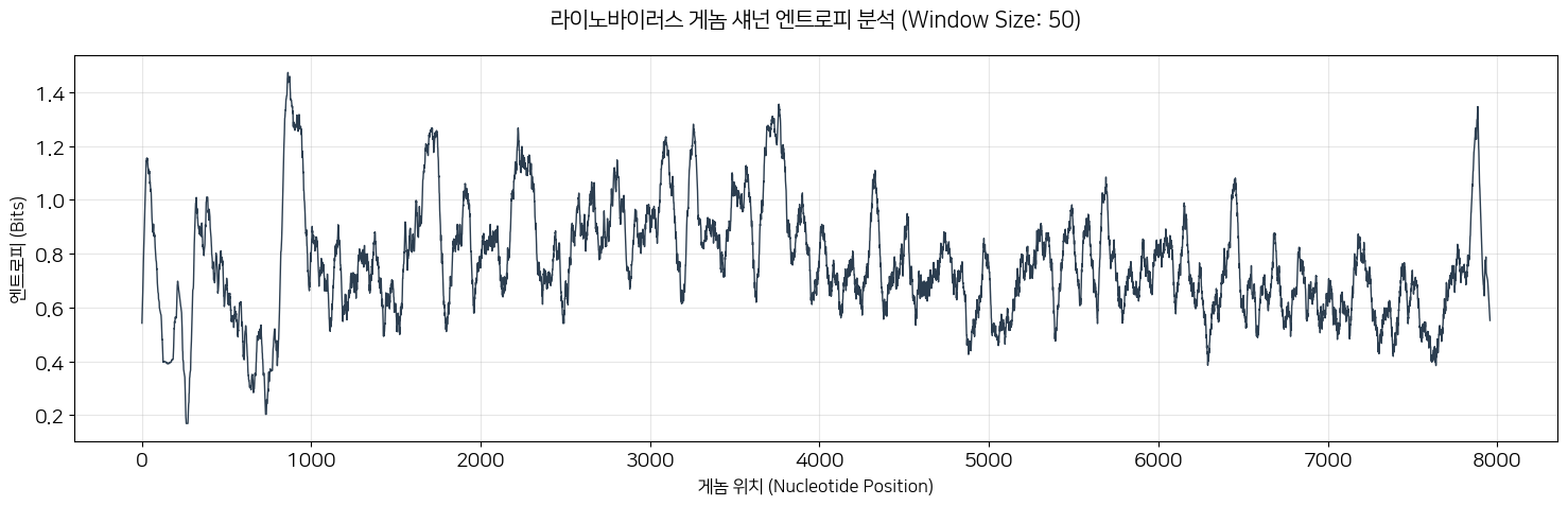
한타때는 뭔 시뻘건 잔디같은거 하나 있었죠? 걔는 잔디 높이가 높을수록 변이가 잘 되는 지역이었고 쟤는 피크가 위로 솟을수록 변이가 잘 되는 구역인겁니다. 보시면 피크가 들쭉날쭉하죠? 그리고 저기 수상학 낮은 부분도 보이죠? 그죠. 쟤들도 아무데나 변이하면 X되는거예요.
# 여러분 이것도 통계분석이 됩니다.
variation_scores = np.array(entropy_values)

mean_var = np.mean(variation_scores)
median_var = np.median(variation_scores)
iqr_var = np.percentile(variation_scores, 75) - np.percentile(variation_scores, 25)

print(f"Mean variation score: {mean_var:.4f}")
print(f"Median variation score: {median_var:.4f}")
print(f"IQR: {iqr_var:.4f}")
Mean variation score: 0.7691
Median variation score: 0.8701
IQR: 1.2085순서대로 평균, 중앙값, 사분위수. 저거 얼로 쏠렸구만...
# Define high-variation hotspots (top 10%)
threshold = np.percentile(variation_scores, 90)

hotspots = variation_scores[variation_scores >= threshold]
non_hotspots = variation_scores[variation_scores < threshold]

u_stat, p_value = mannwhitneyu(
    hotspots,
    non_hotspots,
    alternative="greater"
)

print(f"Hotspot threshold (90th percentile): {threshold:.4f}")
print(f"Mann–Whitney U statistic: {u_stat:.1f}")
print(f"p-value: {p_value:.4e}") # 아 이거는 제가 소수점 조절을 못했어요... 하면 큰일나...
Hotspot threshold (90th percentile): 1.5942
Mann–Whitney U statistic: 5708114.0
p-value: 0.0000e+00그… 피밸류가 이게 맞아요…?
# 변이 점수 분포 히스토그램 (NanumSquare 적용)
plt.figure(figsize=(10, 6))
plt.hist(variation_scores, bins=50, color='#34495e', edgecolor='white', alpha=0.8)

# 통계 지표 수직선 표시
plt.axvline(mean_var, color='red', linestyle='dashed', linewidth=1, label=f'Mean: {mean_var:.4f}')
plt.axvline(median_var, color='orange', linestyle='dashed', linewidth=1, label=f'Median: {median_var:.4f}')

plt.title('라이노바이러스 변이 점수 분포 (Entropy Distribution)', fontsize=15)
plt.xlabel('Variation Score (Entropy)', fontsize=12)
plt.ylabel('Frequency', fontsize=12)
plt.legend()
plt.grid(axis='y', alpha=0.3)
plt.show()
음... 쏠렸어... 이븐하지 아니해...
Phylogenic tree
# 1. 거리 행렬 계산 (Identity 모델 사용)
calculator = DistanceCalculator('identity')
dm = calculator.get_distance(alignment)

# 2. Neighbor-Joining(NJ) 트리 생성
constructor = DistanceTreeConstructor(calculator, 'nj')
tree = constructor.build_tree(alignment)
tree.root_at_midpoint() # 루트를 중간으로 잡아 균형 잡힌 트리 생성

# 3. 시각화 (NanumSquare 폰트가 이미 글로벌 설정되어 있으므로 바로 출력!)
fig = plt.figure(figsize=(12, 8), dpi=100)
ax = fig.add_subplot(1, 1, 1)
plt.title("Rhinovirus Phylogenetic Tree (Based on Whole Genome)", fontsize=18, pad=20)

# Bio.Phylo를 이용한 트리 드로잉
Phylo.draw(tree, axes=ax, do_show=False, label_func=lambda n: str(n) if n.is_terminal() else "")

# 후처리: 축 숨기기 등 깔끔하게 정리
plt.axis('off')
plt.tight_layout()
plt.show()
나도 저거 이름으로 바꾸고 싶은데... 제미나이랑 같이 뭔 짓을 해봐도 안바껴...
def pairwise_identity(seq1, seq2):
    matches = sum(a == b for a, b in zip(seq1, seq2) if a != '-' and b != '-')
    length = sum(a != '-' and b != '-' for a, b in zip(seq1, seq2))
    return matches / length if length > 0 else 0

def extract_clades(tree, cutoff=0.05):
    clade_map = {}
    clade_id = 0

    for clade in tree.find_clades():
        if clade.branch_length and clade.branch_length > cutoff:
            terminals = clade.get_terminals()
            for t in terminals:
                clade_map[t.name] = f"Clade_{clade_id}"
            clade_id += 1

    return clade_map
clade_map = extract_clades(tree, cutoff=0.05)

# ID 정규화 (이거 중요)
normalized_clade_map = {}
for k, v in clade_map.items():
    normalized_clade_map[k.split('.')[0]] = v
within_clade = []
between_clade = []
for rec1, rec2 in combinations(alignment, 2):
id1 = rec1.id.split('.')[0]
id2 = rec2.id.split('.')[0]
if id1 not in normalized_clade_map or id2 not in normalized_clade_map:
continue
identity = pairwise_identity(str(rec1.seq), str(rec2.seq))
if normalized_clade_map[id1] == normalized_clade_map[id2]:
within_clade.append(identity)
else:
between_clade.append(identity)
print(len(within_clade), len(between_clade))u, p = mannwhitneyu(
within_clade,
between_clade,
alternative="greater"
)
print(f'U-statistic: {u:.1f}')
print(f'p-value: {p:.4e}') # 그... 이게... 맞아요?아 위 블록 안주냐고요? 저거 걍 길이라 의미 없음. 맨 휘트니나 보고 가십쇼.
U-statistic: 99900.0
p-value: 4.4644e-84
0은 아니구나… 허허…
effect_size = (
    np.median(within_clade) - np.median(between_clade)
)

print(f'effect_size: {effect_size:.4f}')
n1 = len(within_clade)
n2 = len(between_clade)
rbc = 1 - (2 * u) / (n1 * n2)
print(f"Rank-biserial r: {rbc:.4f}")effect_size: 0.3865
Rank-biserial r: -0.9867r 저거 20개 달았을때는 1떴는데?
'Coding > Python' 카테고리의 다른 글
| M1V1 = M2V2 (0) | 2026.02.15 |
|---|---|
| 코로나바이러스 MSA (0) | 2026.02.05 |
| 식물 데이터도 분석이 되나요? (0) | 2026.01.27 |
| 매우 주관적인 씨본 컬러맵 고르는 방법 (0) | 2026.01.26 |
| 포켓몬과 이항분포 (0) | 2026.01.21 |