참고로 말씀드리는거지만... 분량 ㄹㅇ 역대급임... 노션으로 거의 팔만대장경 나온 듯.
데이터 관련된 얘기는 다른 글에서 다루겠습니다.
install.packages("ggplot2")혹시나... ggplot2가 껄려있지 않다...
깔고 오세요...
> library(ggplot2)어디가요 깔았으면 불러여지.
본인은 저기다가 아예 디렉토리까지 고정으로 박고 시작했다.
나 저 geom 자꾸 점으로 읽어... 클났음...
아무튼! 막대그래프를 그릴 때 쓸 공공데이터는 제주도의 야채 생산 현황에 대한 공공데이터이다.
연산 채소구분대분류 채소구분소분류 면적.ha. 생산량.톤. 조수입.백만원.
1 20-21       노지채소         월동무     5056     359575         106434
2 20-21       노지채소         양배추     1753     103222          60116
3 20-21       노지채소           당근     1357      49527          46108
4 20-21       노지채소         구마늘     1600      24427          85234
5 20-21       노지채소         잎마늘       65       2665           3212
6 20-21       노지채소      양파_조생      524      32735          32596
  데이터.기준일
1      20210809
2      20210809
3      20210809
4      20210809
5      20210809
6      20210809
이건데 한꺼번에 그래프 그리기는 힘들어서
> data_noji=subset(data,채소구분대분류=="노지채소")
> head(data_noji)
   연산 채소구분대분류 채소구분소분류 면적.ha. 생산량.톤. 조수입.백만원.
1 20-21       노지채소         월동무     5056     359575         106434
2 20-21       노지채소         양배추     1753     103222          60116
3 20-21       노지채소           당근     1357      49527          46108
4 20-21       노지채소         구마늘     1600      24427          85234
5 20-21       노지채소         잎마늘       65       2665           3212
6 20-21       노지채소      양파_조생      524      32735          32596
  데이터.기준일
1      20210809
2      20210809
3      20210809
4      20210809
5      20210809
6      20210809
> data_siseol=subset(data,채소구분대분류=="시설채소")
> head(data_siseol)
    연산 채소구분대분류 채소구분소분류 면적.ha. 생산량.톤. 조수입.백만원.
20 20-21       시설채소           상추       12        354           1593
21 20-21       시설채소           깻잎       16        478           3537
22 20-21       시설채소           오이       19        728           1165
23 20-21       시설채소     방울토마토       32       1201           4804
24 20-21       시설채소     일반토마토       19       1451           2903
25 20-21       시설채소           딸기       39       1385          14127
   데이터.기준일
20      20210809
21      20210809
22      20210809
23      20210809
24      20210809
25      20210809
노지채소와 시설재배로 세트 나눠서 했다.
데이터 받는 곳은 나중에 알려드림... 참고로 이거말고 세개 더 받았는데 언어가 깨져서 R에서 못 불러옵디다. 인코딩 다른거는 이해하겠는데 UTF-8에서 깨지는 건 좀 심한거 아니냐...
데이터 분석 일을 하고 있는 김후추씨. (전에도 말했지만 실제로 본인 포켓몬 이름임) 어느 날 출장을 갔던 김후추씨는 보스로라가 어떻게 출장을 가지 도청에서 일하던 신입 데이터 분석가의 고충을 듣게 된다.
"채소 데이터를 분석해서 그래프로 그려오라는데, 리브레오피스가 너무 버벅거려서 그래프를 그릴 수가 없어요. 어떻게 하죠? " (리브레오피스 실제로도 버벅거림 엄청나서 본인은 csv파일도 gedit으로 연다)
> ggplot(data=data_siseol,aes(x=채소구분소분류,y=생산량.톤.,fill=생산량.톤.))+geom_bar(stat="identity")뭘 고민해 R 쓰면 되지.

근데 그래프가 이렇게 돼 있으니까 좀 거시기하네.
> ggplot(data=data_siseol,aes(x=채소구분소분류,y=생산량.톤.,fill=채소구분소분류))+geom_bar(stat="identity")
한결 낫다 그죠?
> ggplot(data=data_siseol,aes(x=채소구분소분류,y=생산량.톤.,fill=채소구분소분류))+geom_bar(colour="black",stat="identity")+ggtitle("제주도 시설재배 야채 생산량") + xlab("채소구분 소분류") + ylab("생산량(톤)")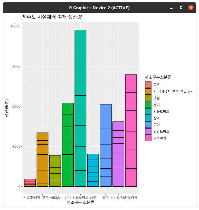
......테두리는 떼버리세요. 안이뻐요.
아, 참고로 막대그래프는 막대 포지션 옵션으로 닷지를 안 주면 누적된다. (막대가 누적된다)
> data2=read.csv('bradford.csv')
> data2
  BSA.conc.mg. OD5951 OD5952 OD5953
1            0  0.001  0.000  0.000
2          200  0.250  0.255  0.241
3          400  0.359  0.400  0.354
4          600  0.550  0.600  0.601
5          800  0.770  0.780  0.755
가상의 Bradford assay 데이터이다. 이게 뭐 하는 분석인지는 나중에 알려드림. 아무튼 저걸로 꺾은선그래프를 그리려면 평균 데이터가 있어야 한다.
> data2$average=round(rowMeans(data2[,c('OD5951','OD5952','OD5953')]),3)
> data2
  BSA.conc.mg. OD5951 OD5952 OD5953 average
1            0  0.001  0.000  0.000   0.000
2          200  0.250  0.255  0.241   0.249
3          400  0.359  0.400  0.354   0.371
4          600  0.550  0.600  0.601   0.584
5          800  0.770  0.780  0.755   0.768
그냥 추가했더니 소수점 개판이라 Round 줘버림...
한참 실험수업을 듣고 있는 제육쌈밥(대짱이). 오늘의 실험은 Bradford assay였다. 조별로 Bardford assay 시약을 처리한 다음 OD595(컬럼이 좀 개판났는데 OD595가 맞음... 세 번 달아서 1, 2, 3이다.)를 측정하고 결과값을 받았다. 과제로 Standard curve를 그려오라는 과제를 받은 제육쌈밥군... 까짓거 후다닥 해치우자! 라고 생각했으나 문제가 생겼다.
제육쌈밥군의 컴퓨터는 리눅스였고, 리브레오피스가 그날따라 매우 버벅였다는 것... 돌릴 수 있는 것은 R밖에 없는데, 이를 어쩌지?
> ggplot(data=data2,aes(x=BSA.conc.mg.,y=average,group=1))+geom_line()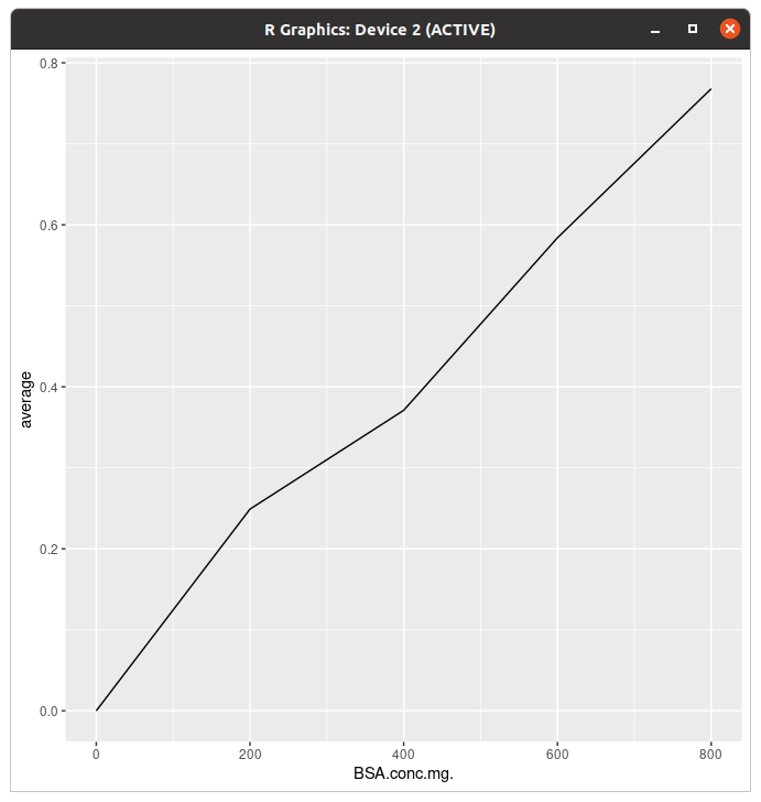
이렇게 하면 일단 그래프는 그려졌는데... 아 라벨 저거 뭐임?
> ggplot(data=data2,aes(x=BSA.conc.mg.,y=average,group=1))+geom_line(colour="#00418c")+geom_point()+xlab("BSA concentration")+ylab("OD595")+ggtitle("Standard curve")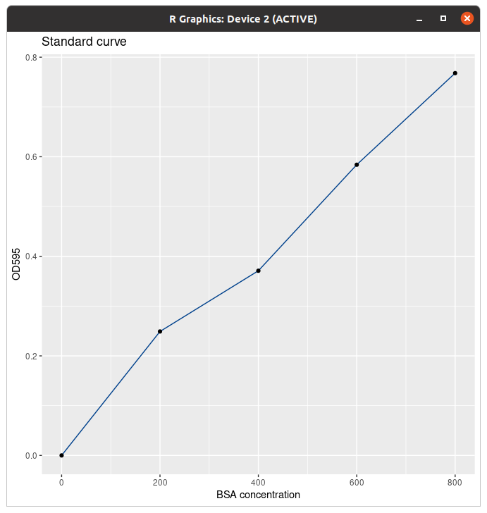
라벨을 바꾸고 제목 추가하고 점(...) 넣고 선을 바꿨다. 사실 저기에 R^2랑 식도 들어가는 게 맞는데 그것까지 하는 법은 나중에 알려드림. 근데 R에서 그게 되나
> ggplot(data=data3,aes(x=Date,y=price,group=time,colour=time,shape=time))+geom_line()+geom_point(size=4)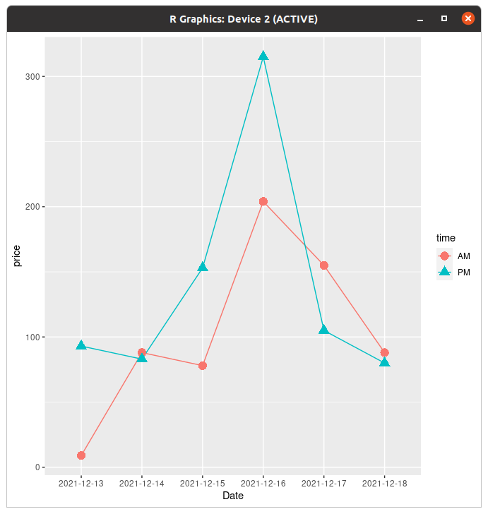
꺾은선그래프는 선별로 색깔을 다르게 주는 것과 동시에 점도 다르게 줄 수 있다.
> ggplot(data=data3,aes(x=Date,y=price,group=time,colour=Date,shape=time))+geom_line()+geom_point(size=4)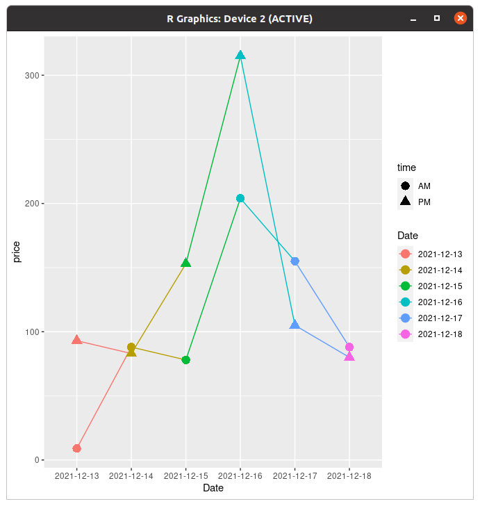
이건 왜 되는거지... (참고로 저 데이터 저번주 무트코인 차트임)
논문에 있는 그래프를 보면 I자같이 생긴 게 있는데 그게 오차막대다. 보통은 표준편차 구해서 넣는다. (표준편차가 범위)
참고로 얘네 함수 정의해서 표준편차 구했는데 함수 없이 구할 수 있으면 그래도 된다. 여기서는 어떻게든 표준편차를 구했다는 전제 하에 진행한다. 안그러면 분량 길어져서 여러분들 스크롤하다 혈압오름...
> ggplot(data=tgc,aes(x=dose,y=len,colour=supp))+geom_line()+geom_point()이거는 단순히 그래프 그려주는 코드.
> ggplot(data=tgc,aes(x=dose,y=len,colour=supp))+geom_line()+geom_point()+geom_errorbar(aes(ymin=len-ci,ymax=len+ci),width=.1)
# Use 95% confidence interval instead of SEM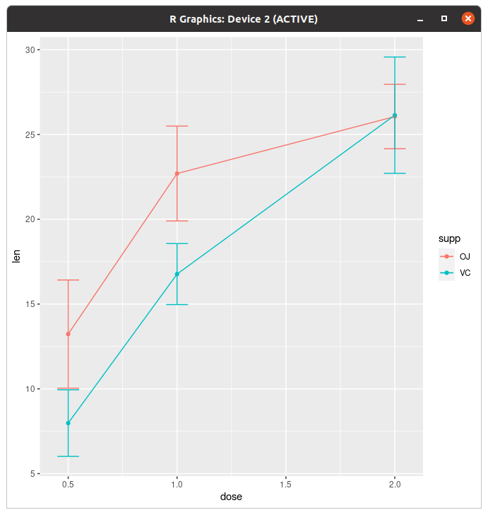
이게 에러바 그려주는 코드다. 코드에
aes(ymin=len-ci,ymax=len+ci)이 부분을 len-sd, len+sd로 해 주면 표준편차로 그릴 수 있다.
> ggplot(data=tgc,aes(x=dose,y=len,colour=supp))+geom_line()+geom_point()+geom_errorbar(aes(ymin=len-ci,ymax=len+ci),colour="black",width=.1)
근데 에러바는 보통 깜장이죠?
> ggplot(data=tgc,aes(x=dose,y=len,colour=supp))+geom_line()+geom_point()+geom_errorbar(aes(ymin=len-se,ymax=len+se),colour="black",width=.1)+expand_limits(y=0)+scale_y_continuous(breaks=0:20*4)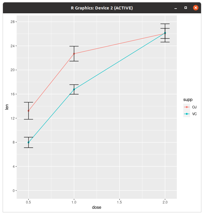
y축 범위 조절하면 에러바도 줄어든다.
막대그래프도 별로 다를 건 없다.
> ggplot(tgc2,aes(x=dose,y=len,fill=supp))+geom_bar(stat="identity",position=position_dodge())+geom_errorbar(aes(ymin=len-se,ymax=len+se),width=.2,position=position_dodge(.9))+scale_y_continuous(breaks=0:20*4)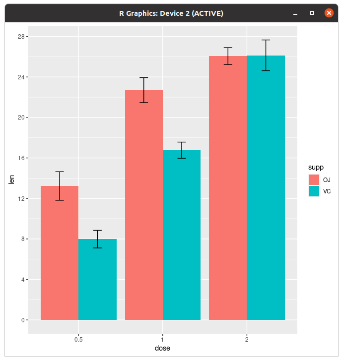
아, 저기서 position=dodge()를 안 주면

막대그래프가 이렇게 된다. 이게 무슨 저세상 누적이여... 아니 이런걸 일일이 해줘야되냐고
점_히스토그램 무엇... 아니 니네 약어 안쓰냐고...
> set.seed(1)
> dat=data.frame(comd=factor(rep(c("A","B"),each=200)),rating=c(rnorm(200),rnorm(200,mean=.8)))
역사와 전통에 의거, 히스토그램은 랜덤 데이터 만들어서 정규분포 곡선 그리는 게 국룰이다. 누가 그러디 내가
> ggplot(dat,aes(x=rating))+geom_histogram()
`stat_bin()` using `bins = 30`. Pick better value with `binwidth`.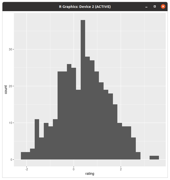
아, 이게 디폴트다.
> ggplot(dat,aes(x=rating))+geom_density()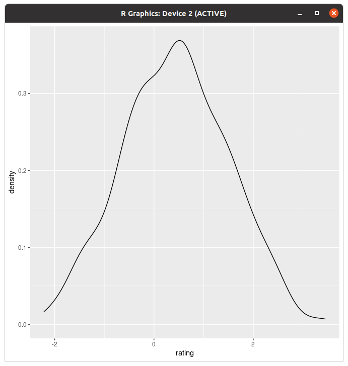
이건 평범한 밀도곡선.
> ggplot(dat,aes(x=rating))+geom_histogram(aes(y=..density..),binwidth=.5,colour="black",fill="#939597")+geom_density(alpha=.2,fill="#f5df4d")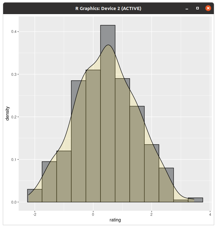
이렇게 하면 겹치는 것도 된다.
> ggplot(dat,aes(x=rating))+geom_histogram()+geom_vline(aes(xintercept=mean(rating,na.rm=TRUE)))
`stat_bin()` using `bins = 30`. Pick better value with `binwidth`.
평균에 선도 그어준다. (밀도곡선도 된다)
근데 사람이 살다보면 복식 히스토그램 그릴 수도 있잖아요! 예 그렇죠.
> ggplot(dat,aes(x=rating,fill=comd))+geom_histogram(binwidth=.5,alpha=.5,position="identity")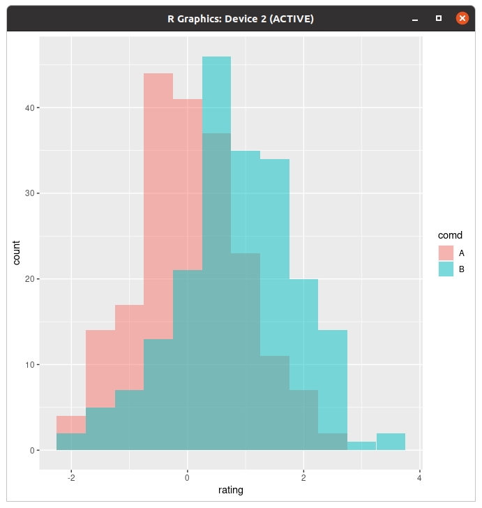
이렇게 투명도를 줘서 겹쳐 그리는 방법도 있고
> ggplot(dat,aes(x=rating,fill=comd))+geom_histogram(binwidth=.5,alpha=.5,position="dodge")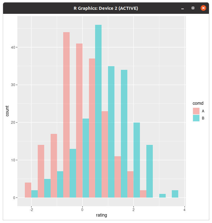
이렇게 닷지로 그리는 법도 있다. 개인적으로는 전자요.
> ggplot(dat, aes(x=rating, fill=comd)) + geom_density(alpha=.3)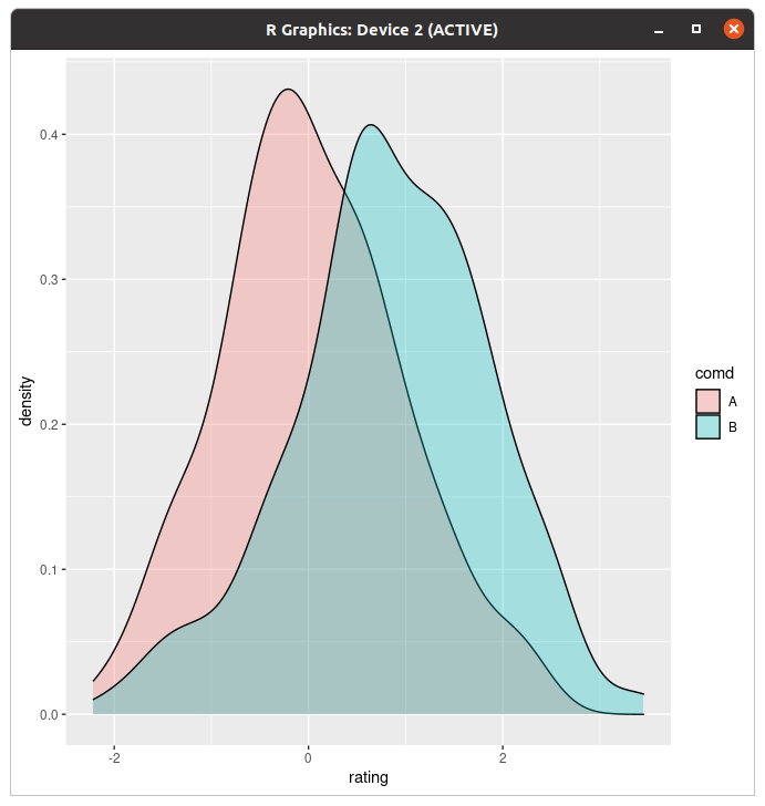
물론 밀도곡선도 된다.
> library(plyr)
> cdat=ddply(dat,"comd",summarise,rating.mean=mean(rating))
> ggplot(dat,aes(x=rating,fill=comd))+geom_histogram(binwidth=.5,alpha=.5,position="dodge")+geom_vline(data=cdat,aes(xintercept=rating.mean,colour=comd))
개별로 선 긋는것도 된다. (왜)
> ggplot(dat, aes(x=rating)) + geom_histogram(binwidth=.5, colour="black", fill="white") +
+     facet_grid(comd ~ .)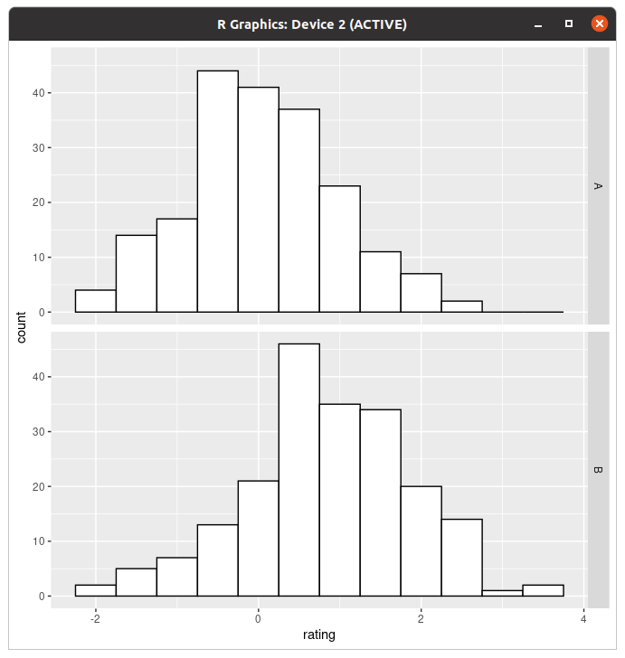
이거는 Facet 파트에서 자세하게 설명할건데 이것도 된다.
> ggplot(dat, aes(x=comd, y=rating)) + geom_boxplot()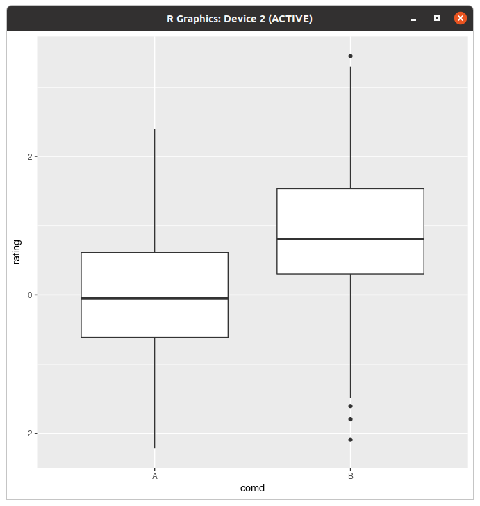
평범한 box plot은 이렇게 생겼다.
> ggplot(dat, aes(x=comd, y=rating,fill=comd)) + geom_boxplot()+coord_flip()
그래서 눕혀드렸습니다^^ (coord_flip=xv축 값을 바꾼다)
> ggplot(dat, aes(x=comd, y=rating,fill=comd)) + geom_boxplot()+stat_summary(fun.y=mean,geom="point",size=3,shape=5)
경고메시지(들):
`fun.y` is deprecated. Use `fun` instead.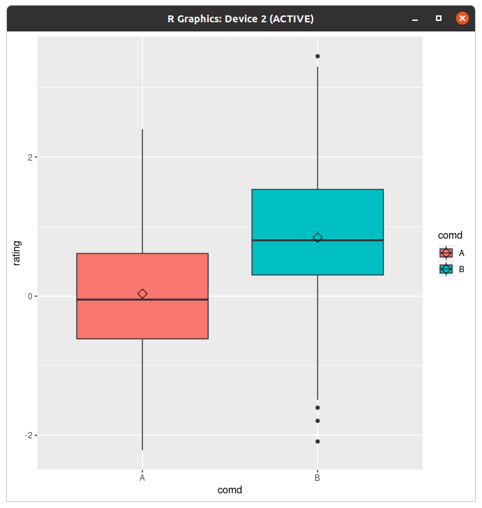
아 평균도 찍어준다니까요
저 포인트 꺾은선에서 본 것 같다고? 쟤는 라인이랑 둘이 쓰면 꺾은선 그래프에 점 찍어주고, 단독으로 쓰면 산점도다.
참고로 예전에 python 하면서도 설명했나 모르겠는데 산점도는 XY축 값이 다 있어야 한다.
> dat <- data.frame(cond = rep(c("A", "B"), each=10),
+                   xvar = 1:20 + rnorm(20,sd=3),
+                   yvar = 1:20 + rnorm(20,sd=3))
> dat
   cond         xvar         yvar
1     A -4.252354091  3.473157275
2     A  1.702317971  0.005939612
3     A  4.323053753 -0.094252427
4     A  1.780628408  2.072808278
5     A 11.537348371  1.215440358
6     A  6.672130388  3.608111411
7     A  0.004294848  7.529210289
8     A  9.971403007  6.156154355
9     A  9.007456032  8.935238147
10    A 11.766997972  8.928092187
11    B  8.840215645 13.202410972
12    B  5.974093783 17.644890794
13    B 15.034828849 10.485402010
14    B 10.985009895 10.138043066
15    B 13.543221961 18.681876114
16    B 11.435789493 19.143471805
17    B 16.977063388 18.832504955
18    B 17.220012698 18.939818864
19    B 17.793359218 19.718587761
20    B 19.319909163 19.647899863
그래서 난수가 1+1이 되었습니다.
> ggplot(dat,aes(x=xvar,y=yvar))+geom_point(shape=1)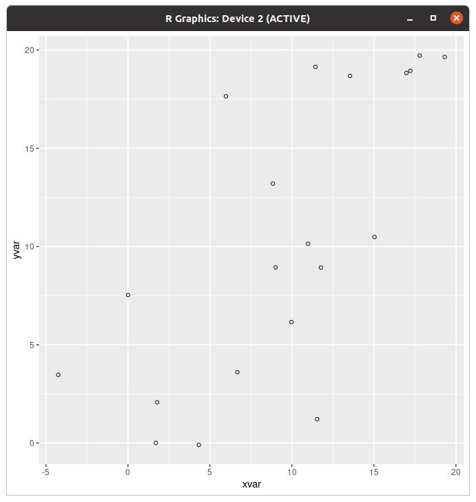
펑범한 산점도
> ggplot(dat,aes(x=xvar,y=yvar))+geom_point(shape=5)+geom_smooth(method=lm,se=FALSE)
`geom_smooth()` using formula 'y ~ x'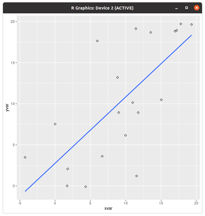
에 regression line을 얹어서 드셔보세요! 그거 먹는거 아냐
> ggplot(dat,aes(x=xvar,y=yvar))+geom_point(shape=5)+geom_smooth(method=lm)
`geom_smooth()` using formula 'y ~ x'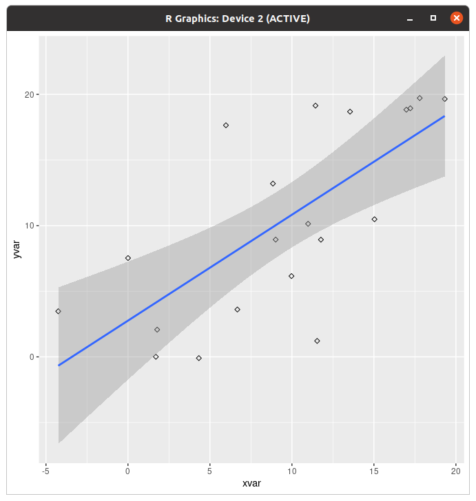
뭔지 모르겠는것도 같이 말아서 드셔보세요!
> ggplot(dat,aes(x=xvar,y=yvar))+geom_point(shape=5)+geom_smooth()
`geom_smooth()` using method = 'loess' and formula 'y ~ x'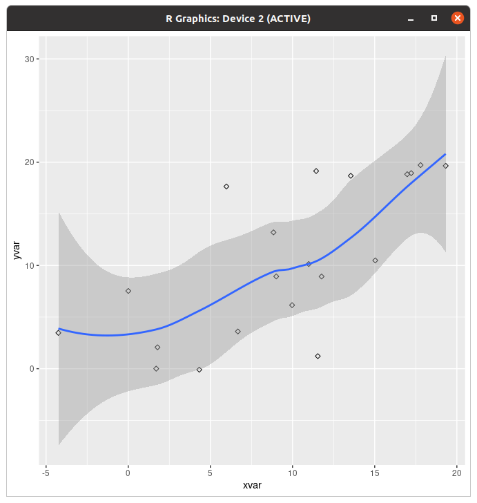
이거 뭔데 애가 흐물흐물해짐???
근데 사람이 살다보면 산점도를 막 그룹별로 그리기도 한다 그죠?
> ggplot(dat,aes(x=xvar,y=yvar,color=cond))+geom_point(size=3)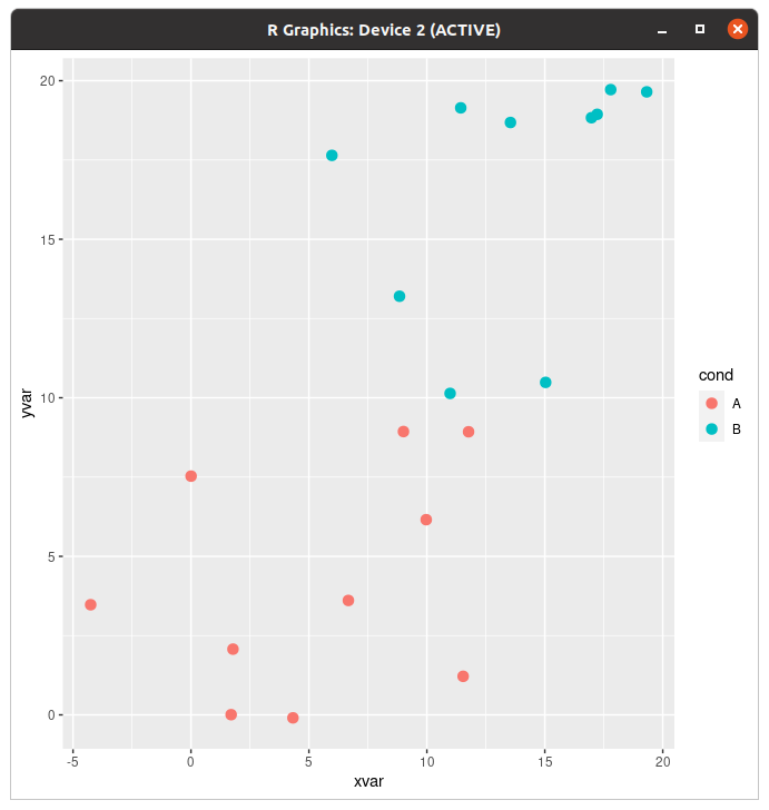
그렇다고
> ggplot(dat,aes(x=xvar,y=yvar,color=cond))+geom_point(size=3)+scale_color_manual(values=c("#f5df4d","#939597"))+geom_smooth(method=lm,se=FALSE)
`geom_smooth()` using formula 'y ~ x'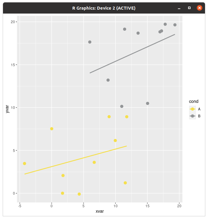
> ggplot(dat,aes(x=xvar,y=yvar,color=cond))+geom_point(size=3)+scale_color_manual(values=c("#f5df4d","#939597"))+geom_smooth(method=lm,se=FALSE,fullrange=TRUE)
`geom_smooth()` using formula 'y ~ x'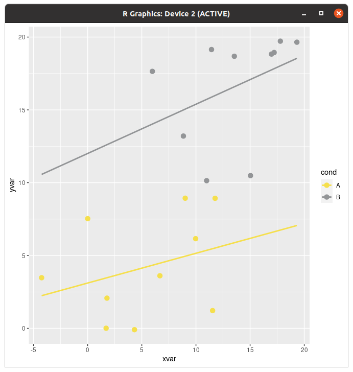
아 회귀곡선도 낭낭하게 따로 넣어드린다니까요
> ggplot(dat,aes(x=xvar,y=yvar,shape=cond,color=cond))+geom_point(size=3)
아 점 모양도 낭낭하게 바꿔드린다니까요
오버플로팅이 뭔지는 모르겠으나
> dat$xrnd=round(dat$xvar/5)*5
> dat$yrnd=round(dat$yvar/5)*5
> ggplot(dat,aes(x=xrnd,y=yrnd))+geom_point()
반올림했더니 그래프가 뭐야 내 산점도 돌려줘요가 될 때가 있다.
> ggplot(dat,aes(x=xrnd,y=yrnd))+geom_point(alpha=1/4)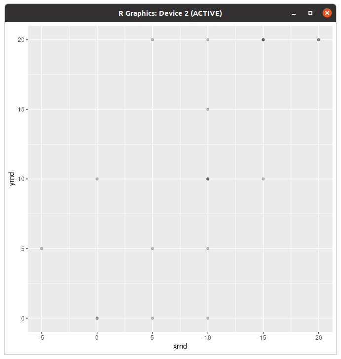
점에 알파를 줘 보면 겹친 영역에 따라 색이 다른 것이 보인다. (진한색이면 거기 겹쳐진 게 많은 거)
> ggplot(dat,aes(x=xrnd,y=yrnd))+geom_point(size=3,position=position_jitter(width=1,height=.5))
닷지 줘도 대충 보이시져?
| R의 내장 데이터 (부제: 공공데이터 어떻게 받아요?) (0) | 2022.08.22 |
|---|---|
| R 배워보기-8.1. ggplot2로 그래프 그리기 (하) (0) | 2022.08.22 |
| R 배워보기-7. Statistical analysis (하) (0) | 2022.08.21 |
| R 배워보기-7. Statistical analysis (상) (0) | 2022.08.21 |
| R 배워보기- 6.5. Manipulating data-Sequential data (0) | 2022.08.20 |


